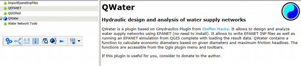
Bakgrund
Dimensioneringen av trycksatta vattenledningar är en komplex uppgift som kräver noggrann analys av flera faktorer, inklusive flöde, tryckfall, rörmaterial och topografi. QWater har utvecklats för att underlätta denna process och ge ingenjörer och planerare ett kraftfullt verktyg för att optimera vattenledningssystem.
Funktioner
1. Hydraulisk Beräkning
QWater använder avancerade hydrauliska beräkningar för att analysera flöde och tryckfall genom vattenledningssystemet. Genom att ta hänsyn till variabler som rördiameter, material och topografi, genererar QWater noggranna resultat för att säkerställa optimal prestanda.
2. Användarvänligt Gränssnitt
QWater erbjuder ett intuitivt gränssnitt som möjliggör enkel navigering och användning. Med ett användarvänligt gränssnitt kan användare enkelt mata in och justera parametrar för att snabbt få resultat och visualiseringar.
3. Automatiserad Optimering
Genom att utnyttja avancerade algoritmer för optimering kan QWater automatiskt föreslå de mest effektiva rördimensionerna och andra parametrar för att möta specificerade krav. Detta sparar tid och resurser samtidigt som det säkerställer optimal prestanda.
Användarmanual
För att använda QWater effektivt, följ dessa steg:
- Inmatning av Data: Ange nödvändiga data såsom flöde, tryckkrav, rörmaterial och topografisk information.
- Beräkning: Kör hydrauliska beräkningar genom att använda QWaters inbyggda motor.
- Optimering: Om så önskas, låt QWater föreslå optimerade parametrar för att uppnå önskad prestanda.
- Visualisering: Granska och analysera resultatet genom QWaters grafiska gränssnitt.
- Rapportering: Generera och exportera detaljerade rapporter för att dokumentera och dela dimensioneringsresultaten.
Utökning av Funktionalitet – Testning av Trycksatta Ledningar vid Nätverksanslutning och överför ledningsnät till Civil3D
Utöver dimensioneringen av vattenledningar erbjuder QWater möjligheten att testa trycksatta ledningar när de ansluts till det befintliga ledningsnätet. Denna funktion säkerställer att den planerade anslutningen integreras sömlöst med det befintliga nätverket och uppfyller önskade flöde- och tryckkrav. Här är hur du kan använda den här funktionen:
1. Lägg till Anslutningspunkter:
- Ange specifika anslutningspunkter där det nya ledningsnätet kommer att anslutas till det befintliga nätverket.
- Importera dimensionerad ledningsnät från QGIS till Civil3D, använd MAPIMPORT och konvertera MAP-ledningar till Civil3D-pipes med kommando: ”map_get_pw”
2. Konfigurera Flöde och Tryck:
- Ange önskat flöde och tryck för det nya ledningsnätet vid anslutningspunkterna. Detta kan vara baserat på systemkrav eller projektspecifikationer.
- Välj ledningsnät för beräkning av ledningstryck i högsta tappställe
3. Iterativ Process:
- Vid behov kan processen upprepas med olika parametrar eller anslutningspunkter för att hitta den mest optimala lösningen.
Prepare QGIS
- Create a new Qgis project
- Adjust the project coordinate system for Sirgas 2000, in the meridian range of the area where the network will be designed (for example for Salvador – EPSG: 31984).
- Create shapes for the types of elements that make up the network (using the same project coordinate system):
- Points: Nodes, Reservoirs and pumps (if any).
- From lines: excerpts
- Save the project
- Import the planimetric base to be used
- Relate the created shapes to the Epanet information types (Plugins/ Qwater / Settings>)
- Junctions = Nodes
- Pipes = Segments
- Reservoirs = Reservoirs
- At this stage take the opportunity to input the initial and final population for the network to be analysed.
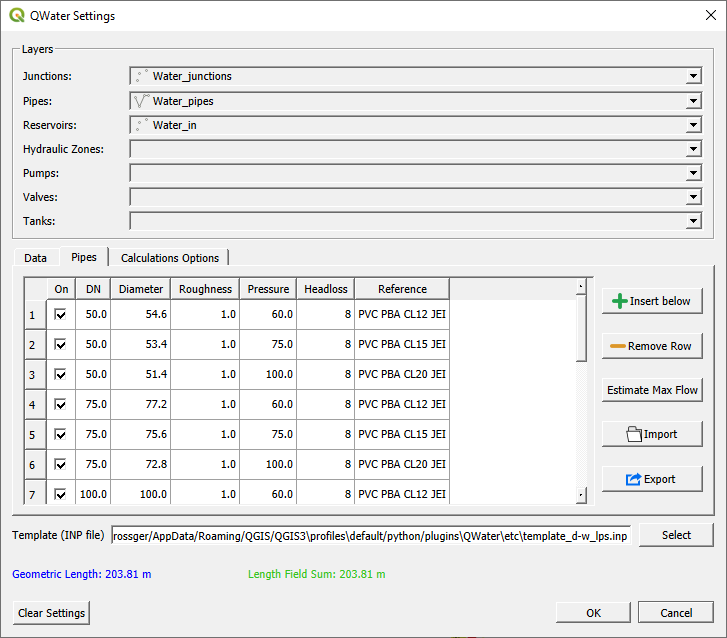
- Under the ”Pipes” tab insert the relevant pipe properties for the respective pipe diameters and materials
- In the ”Calculations Options” tab, set the maximum allowed velocity (default = 5 m/s) and check Calculate pipe length
- Click the ”Select” button and choose the ”template_d-w_lps.inp” calculation configuration
- Click Plugins / Qwater / Make model and accept all messages
- For all shapes, save and exit edit mode
- Click in <Project / Snapping Options> and click on the magnet icon (to enable snapping).
Mapping the Network
Reservoir
- Select the shape of reservoirs and click on the edit button
- Enable the layer label to display the ”DC_ID” field
- Locate all reservoirs (fixed level) by filling the ”HEAD” field with the Water Elevation (Ground Elevation + Reservoir height). Open the table to verify that all reservoirs have values in the HEAD field.
- Change the display of the label to ==> ’Node:’ || ”DC_ID” || ’\ n Elevation =’ || ”HEAD”
- Save the shape and exit edit mode
Nodes
- Select the node shape and click the edit button
- Enable the layer label to display the ”DC_ID” field
- Locate all nodes
- Fill in the ”ELEVATION” field with the Terrain Elevation. Open the table to verify that all nodes have values in the ELEVATION field.
- Change the display of the label to ==> ’Node:’ || ”DC_ID” || ’\ n Elevation =’ || ”ELEVATION”
- Save the shape and exit edit mode
Segments
- Select the segments shapes and click on the edit button
- Enable the layer label to display the ”DC_ID” field
- Trace all segments according to the direction of the predicted flow (from upstream to downstream). A excerpt consists of a polyline that starts at the upstream node and ends at the downstream node. Note: Right click to finish. Esc key to cancel the current edit.
- Fill in the attributes tables with default values by click <Plugins / Qwater / Fill up Fields>
- Save the shape and exit edit mode.
Calculating Demand
- Click <Plugins / Qwater / Calc Flow>. The message ”Demand on nodes calculated successfully” should appear. This routine calculates the unit flow from the distributed demand by allocating at each node the product of the unit flow times half the length of the segments connected to the node.
- (Optional) It is also possible to calculate flows based on a Zonal Polygon layer.
- Create a polygon layer and create one polygon for delimit each hydraulic zone (in this case Zone with a especific demand)
- Save the polygon
- Define it as Hydraulic Zone layer by setting in <Plugins/ Qwater / Settings / Hydraulic Zone layer>
- Run <Plugins / Qwater / Make model> and accept all messages to create the necessary attribute table fields
- Fill in the field ’DEMAND’ of each Hydraulic Zone
- Click <Plugins / Qwater / Calc Flow>
- Save the node shape and exit edit mode.
Preliminary Network Simulation
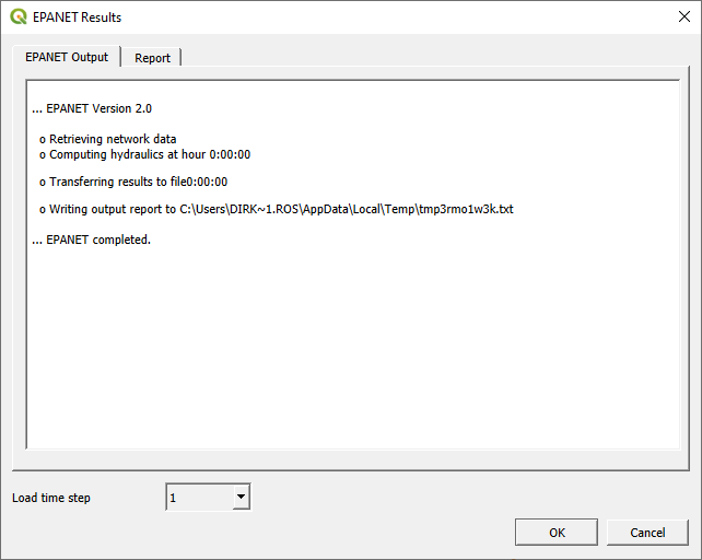
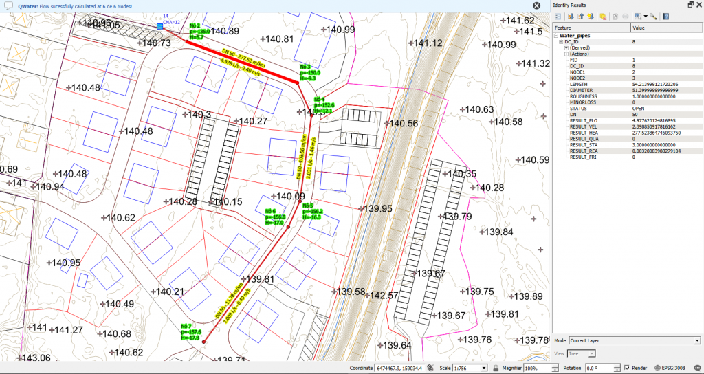
- Click <Plugins / Qwater / Run Epanet Simulation> and wait for the message to be displayed. If the message indicates the occurrence of errors, analyze the error feedback in the ”Report” tab.
- If the simulation was successful, save the shapes and exit the edit mode.
Optimization of the Network Diameters
- Click <Plugins / Qwater / Calculate economics diameter> and confirm the message to replace the values in the ”DIAMETER” field.
- Save shapes and exit edit mode. Note: The used pipe Diameters for optimization are defined in ’Pipe tab’ of the Settings Dialog.
Network simulation with optimized diameters
- Click <Plugins / Qwater / Run Epanet Simulation> and wait for the message to be displayed.
- If the simulation was successful, save the shapes and exit the edit mode.
Final Adjustments
- Save the project
- Save the project (suggestion previous name plus result, eg: Network_result.qgs).
- Click <Plugins / Qwater / Load default Styles>.
- Analyze the results and fine-tune the reservoir HEAD, diameters of segments.
- Run the network simulation again (<Plugins / Qwater / Run Epanet Simulation>)
- Save the shapes and exit edit mode.
- Save the project.
- (Optional) Export the network designed for the dxf format. Adapt a compatible scale.
No responses yet